Back to our Tracker tab. In column A, we’re going to add a drop-down so we can select the client. To do this, highlight A2:A, click Data (in the top bar), then Data Validation. This will pop up a new window.
Within this window, we’re going to update the criteria section. Most of this is already prepared for what we need, we just need to update the target range.
Click the grid within the criteria area, go to the “Clients overview” tab and select A2:A.
Click Save.
Now you have a drop-down containing each of your clients named in the “Clients Overview” tab.
In column F, we are going to add a similar drop-down, but this time based on the stage section in the “Templates” tab. Follow the above steps but for column F, and this time select A2:A in the “Templates” tab as the target range.
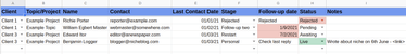
The final drop-down column will be column H. Select Data Validation as above until the additional window opens. Here we are going to change the criteria drop-down to “List of items”. This allows us to add different options to the drop-down manually. In the next box over, add “Pending,Awaiting,Live,Rejected”, then Click Save.
Next up is a switch formula in Column G.
=iferror(SWITCH(F2,”initial”,E2+3,”Follow-up one”,E2+5,”Follow-up two”,E2+7,”Follow-up three”,E2+14,”restart”,E2+180,”personal”,”Check last reply”,”rejected”,”Rejected”),””)
This formula looks at what has been selected (if anything) in column F and performs a calculation based on the selected outreach stage.
Each stage in the drop down on column F is included as an option (this will need to be customised to your specific stages). From here the additional wait time (in days) is added to the last contacted date (column E). Customise the number of wait days to match your outreach process.
Copy this formula down to the last row on the tab.
Conditional Formatting
Now for conditional formatting. We will use this to colour column G one of three colours based on the contents of the cell and today’s date.
Highlight G2:G and click “Format” > Conditional Formatting. This will open a sidebar with some additional options.
Ensure the “Single colour” tab is selected, then use the drop-down (Format Rules > Format Cells if) to select “Date is before”. An additional drop-down will appear – select “Today” from this and change the formatting style to red. This will highlight any contact which is overdue.
Click Done. The sidebar should stay open (if not, re-open using the steps above).
Click “+ Add another rule”.
Follow the steps above, but select “Date is” in the format rules and select yellow for the formatting style. This will highlight any contact which is due today.
Add one last rule with the steps from above, but select “Date is after” in the format rules and select green for the formatting style. This will highlight any contact who does not yet need to be contacted again.
This completes the tracker setup!